Algorithms

Algorithms are multi-step processing pipelines that inherit from Algorithm. They follow the Template Method pattern: the base class handles mixed-precision wrapping, and subclasses implement apply().

Usage Pattern

algo = SomeAlgorithm(device="cuda")
output = image.clone()
algo(image=image, output=output)

mask = output.pixel_data          # result tensor
annotations = output.annotations  # per-lesion annotations (if applicable)

Available Algorithms

Algorithm	Description
FebdsAlgorithm	Fourier Enhancement + Band-pass Detection and Segmentation for microcalcifications
TopHatAlgorithm	White top-hat morphological filtering
KMeansAlgorithm	Hard K-Means clustering segmentation
FCMAlgorithm	Fuzzy C-Means soft clustering
PFCMAlgorithm	Possibilistic Fuzzy C-Means (typicality-based)
BreastMaskAlgorithm	Breast region extraction via Otsu + largest connected component
DicomWindowAlgorithm	Linear DICOM window center / width mapping
GrailWindowAlgorithm	GRAIL perceptual windowing with Gabor-filtered MI
BitDepthNormAlgorithm	Automatic bit-depth detection and normalization
SbrgAlgorithm	Seed-Based Region Growing segmentation
DeepSegmentationAlgorithm	Deep learning segmentation with remote model support

FEBDS (Microcalcification Detection)

The FEBDS algorithm combines enhancement, filtering, thresholding, and morphology into a single pipeline:

from medical_image import FebdsAlgorithm

algo = FebdsAlgorithm(method="dog", device="cpu")
output = image.clone()
algo(image=image, output=output)

mask = output.pixel_data.numpy()

Methods: "dog" (Difference of Gaussians), "log" (Laplacian of Gaussian), "fft" (Fourier band-pass).

Clustering Algorithms

K-Means, FCM, and PFCM segment images by grouping pixels into clusters:

from medical_image import KMeansAlgorithm, PatchGrid, RegionOfInterest

# Normalize and extract a patch for clustering
normalized = RegionOfInterest.normalize(image.clone(), divisor=4095.0)
grid = PatchGrid(normalized, (64, 64))
patch_img = grid.patches[0].to_image()

out = patch_img.clone()
km = KMeansAlgorithm(k=3, device="cpu", random_state=42)
km(patch_img, out)

# Access clustering results
print(km.centroids.shape)  # (3, 1)
print(km.converged)        # True/False
for s in km.stats:
    print(f"Cluster: {s['pixels']} pixels, MC={s['is_mc']}")

Deep Segmentation

Run pretrained deep learning models with automatic download and caching:

from medical_image.algorithms.deep_segmentation import DeepSegmentationAlgorithm

# List available pretrained models
models = DeepSegmentationAlgorithm.list_available_models()
for m in models:
    print(f"{m['name']} - {m['architecture']}, patch={m['patch_size']}")

# Download and load
algo = DeepSegmentationAlgorithm.from_pretrained(
    "unetpp_bce_dice_32_inbreast", device="cuda"
)
print(algo.model_info)  # {'architecture': 'unetpp', 'loss': 'bce_dice', ...}

# Inference
output = image.clone()
algo(image=image, output=output)

# Results
mask_np = output.pixel_data.cpu().numpy()       # binary mask
prob_np = algo.probability_map.cpu().numpy()     # probability map [0, 1]
print(f"Found {algo.lesion_count} lesions")

for ann in output.annotations:
    print(f"  {ann.label}: confidence={ann.metadata['confidence']:.2f}, "
          f"area={ann.metadata['area']}px")

Models are cached in ~/.cache/medical-std/models/.

Visualizing Inference Results

After running inference, the model produces a probability map. To obtain a clean binary mask, threshold the probability map — a threshold of 0.7 reduces false positives compared to the default 0.5:

import matplotlib.pyplot as plt
import numpy as np
import torch
from medical_image import DicomImage
from medical_image.algorithms.deep_segmentation import DeepSegmentationAlgorithm

# Load DICOM
image = DicomImage("mammogram.dcm")
image.load()
if not isinstance(image.pixel_data, torch.Tensor):
    image.pixel_data = torch.from_numpy(image.pixel_data).float()

# Run inference
algo = DeepSegmentationAlgorithm.from_pretrained(
    "unetpp_bce_dice_32_inbreast", device="cuda"
)
output = image.clone()
algo(image=image, output=output)

# Extract arrays
image_np = image.pixel_data.detach().cpu().numpy()
if image_np.max() > 1.0:
    image_np = image_np / image_np.max()

# Threshold probability map at 0.7
prob_np = algo.probability_map.detach().cpu().numpy()
mask_np = (prob_np >= 0.7).astype(np.float32)

# Visualize
fig, axes = plt.subplots(1, 3, figsize=(18, 6))

axes[0].imshow(image_np, cmap="gray")
axes[0].set_title("DICOM Image")
axes[0].axis("off")

axes[1].imshow(mask_np, cmap="gray", vmin=0, vmax=1)
axes[1].set_title("Predicted Mask (threshold = 0.7)")
axes[1].axis("off")

axes[2].imshow(image_np, cmap="gray")
axes[2].imshow(mask_np, cmap="Reds", alpha=0.4, vmin=0, vmax=1)
axes[2].set_title("Segmentation Overlay")
axes[2].axis("off")

plt.tight_layout()
plt.show()

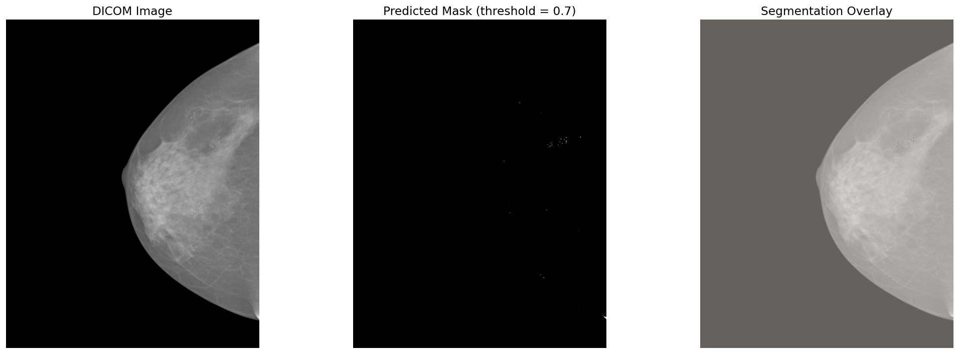
The three panels show: (1) the original DICOM mammogram, (2) the binary mask after thresholding the model output at 0.7, and (3) the mask overlaid on the original image in red to highlight detected regions.

Loading from Local Checkpoint

algo = DeepSegmentationAlgorithm(
    checkpoint_path="results/unet_bce_dice_128_inbreast/best_model.pt",
    device="cpu"
)
# Config (patch_size, clahe, threshold) auto-read from checkpoint

ROI Pipeline: TopHat and FEBDS

A common workflow extracts a region of interest, then applies classical algorithms for microcalcification enhancement:

from medical_image import (
    DicomImage, RegionOfInterest,
    TopHatAlgorithm, FebdsAlgorithm,
)
import matplotlib.pyplot as plt

# Load DICOM and extract ROI around a suspicious region
image = DicomImage("mammogram.dcm")
image.load()

roi = RegionOfInterest.from_center(image, cx=1250, cy=2000, half_size=127)
roi_img = roi.load()
RegionOfInterest.normalize(roi_img, divisor=4095.0)

# TopHat on the ROI (enhances small bright structures)
th_out = roi_img.clone()
TopHatAlgorithm(radius=3, device="cpu")(roi_img, th_out)

# FEBDS on the full image, then extract same ROI
febds = FebdsAlgorithm("dog", device="cpu")
full_out = image.clone()
febds(image=image, output=full_out)

roi_febds = RegionOfInterest.from_center(full_out, cx=1250, cy=2000, half_size=127)
roi_febds_img = roi_febds.load()

# Visualize
fig, axes = plt.subplots(1, 3, figsize=(15, 5))

axes[0].imshow(roi_img.pixel_data.cpu().numpy(), cmap="gray")
axes[0].set_title("ROI (normalized)")
axes[0].axis("off")

axes[1].imshow(th_out.pixel_data.cpu().numpy(), cmap="gray")
axes[1].set_title("TopHat (radius=3)")
axes[1].axis("off")

axes[2].imshow(roi_febds_img.pixel_data.cpu().numpy(), cmap="gray")
axes[2].set_title("FEBDS (DoG)")
axes[2].axis("off")

plt.tight_layout()
plt.show()

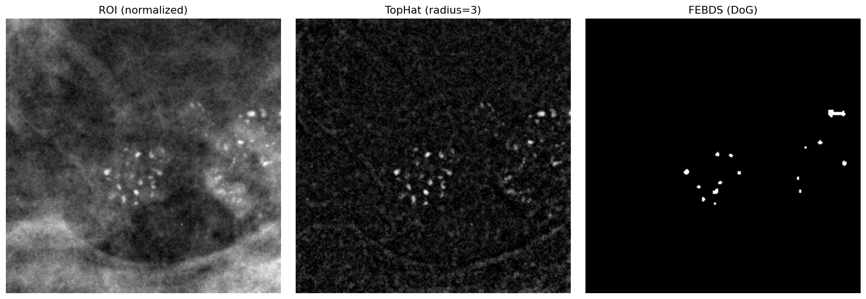
The three panels show: (1) the extracted and normalized ROI from the mammogram, (2) the TopHat-enhanced output that highlights small bright structures like microcalcifications, and (3) the FEBDS algorithm output using Difference of Gaussians for band-pass enhancement.

Breast Mask Extraction

from medical_image import BreastMaskAlgorithm

# Binary mask only
algo = BreastMaskAlgorithm(mask_only=True)
output = image.clone()
algo(image, output)

# Masked mammogram (background removed)
algo = BreastMaskAlgorithm(mask_only=False)
output = image.clone()
algo(image, output)

Composing Algorithms

Build custom pipelines by combining existing operations:

from medical_image.algorithms.algorithm import Algorithm
from medical_image import Filters, Threshold

class MyPipeline(Algorithm):
    def apply(self, image, output):
        # Step 1: Gaussian blur
        Filters.gaussian_filter(image, output, sigma=2.0, device=self.device)

        # Step 2: Otsu threshold
        temp = output.clone()
        Threshold.otsu_threshold(output, temp, device=self.device)

        output.pixel_data = temp.pixel_data
        return output